Sensor modelling

The sensor has been calibrated and therefore it is now possible to use ISET to model the sensor output given a map of reflectance.

First we need to convert a pdf file to a map of cmyk.

We also need to compute the reflectance from any cmyk value.

We can then make a scene in ISET with it.

Finally we model the sensor.

PDF to cmyk:

Description of problem

An important aspect of modeling the printer optical sensor is to accurately model its input. The printing process starts when a user at a computer requests a page to be printed. The specific page is at that time encoded in a high level page description language format such as Postscript (PS), Portable Document Format (PDF) or Encapsulated Postscript (EPS). A raster image processor is responsible in converting this image representation to an image represented in the natural color space of a printer i.e. in converting a PS, PDF or EPS file format to a bitmap file in the CMYK color space. A bitmap file that allows us to represent an image in its CMYK values is the Tagged Image File Format (TIFF). Hence the goal of this stage is to produce the CMYK values for each pixel position, so that they can be used in the next stage to interpolate the reflectance values.

Method used to solve the problem

It is possible to convert a PS, PDF or EPS file to a TIFF file in the CMYK color space following a number of simple steps. Already existing software packages are used to solve this problem, which are free and open source.  

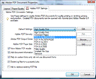
The first thing to note is that in creating the PS, PDF or EPS file format, we need a printing device that is able to do that. For example the Adobe PDF printer can be used, or depending which operating system you are using you might opt for something different. In any case, the printer you are going to use for creating the PS, PDF or EPS file, must give you the option to represent the image in the CMYK color space (for example, the Adobe PDF printer, gives you that option in its advanced settings, see figure 1).  

Figure 1 CMYK color space in Adobe PDF Settings

Another subtlety worth noting is that many printers are black and white, so you would need to find a printing device that prints in all colors. Once you install the printer, and choose the CMYK color space option, you can create the high level page description format of the page you want to print. Let’s assume that you have created a PDF file called test.pdf. The test image is shown in figure 2.

Figure 2 Input PDF file

The software that will make the conversion from a PDF file to a TIFF file requires that ghostscript is installed on the machine. Hence you would need to install ghostcript (http://www.ghostscript.com/). Installation instructions can be found on their website.

The next step is to install the software that will convert the test.pdf to test.tiff. The software that does that is called ImageMagick (http://www.imagemagick.org/). The website contains many versions of the software, depending on what you want to do with ImageMagick. For example, if you only want to use it for its command line programs, you only need to download the binary release. It also supports various operating systems, and you need to choose the one that corresponds to yours. If you are in any doubt you can contact me at any time. If you are using windows you can use the following link to download the software

http://www.imagemagick.org/download/binaries/ImageMagick-6.5.0-2-Q8-windows-static.exe

For further help in installing the software you can either use the website, or contact me.

Once you have installed imageMagick, you can open the command line prompt of your system (if you are using Windows just type cmd in the run window). Navigate to the folder that contains test.pdf and type convert test.pdf test.tiff

Conversion

That’s it. A new file called test.tiff is created. This is the CMYK color space representation of the page.  

You can read this in MatLab using the following command

Im = imread(‘test.tiff’,’tiff’);

CMYK to reflectance models:

We now want to transform the CMYK values obtained by the renderer into estimated reflectance data to simulate our printed paper.

In this purpose, we used the data provided by HP that gives us a measurement of the reflectance at 35 different wavelengths for 1338 different CMYK values.

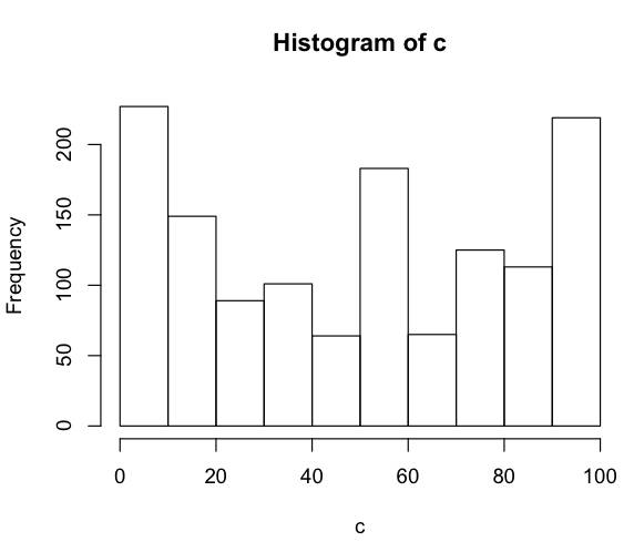
Let's first have a look at the repartition of the data over the CMYK space. Here is the histogram of values for the C values. (We have exactly the same histogram for the M and Y values).

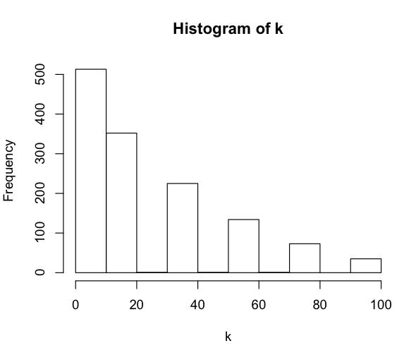
Here is the histogram the the K values:

We can see that the CMYK values provided globally cover the entire space of possibilities even if we have less measurement with value K=100 that we have for K=0. This can be explained by the fact that when K is higher, the color is much darker and changing the other value of C,M and Y do not make much difference in the reflectance estimation.

With this repartition in mind, we developed two models to fit CMYK values in reflectance datas.

1) Nearest neighbor estimation or locally linear model

The first model we developed is a locally linear model that uses nearest neighbors to find the reflectance for a given CMYK value.

Having our entire database of 1338 values, we want to find a reflectance approximation for every possible CMYK values in our space. In this purpose, given a new CMYK value, we will find the nearest neighbors in the database and allocate each of them a weight depending on their euclidian distance to our current value.

Then, computing the reflectance for our current CMYK value consist of averaging the reflectances of the nearest neighbors found with their respective weights.

As we can see from the previous histogram, the database gives us a quite dense representation of the CMYK space, and then, we believe this model is very well suited to approximate correctly the reflectance values from any CMYK value.

As we can see here, we need to keep in memory the entire database to compute the nearest neighbors and then the reflectance estimation. For our study, this is perfectly reasonable but the computation might be too high for a real-time application.

So we also decided to develop a global linear model for fast computation.

2) Log-linear model

Here, we will try to fit a globally linear model on our data to see if we can represent our entire dataset by such a family of models.

Let's consider three wavelengths from our 35 original wavelengths from the database and let's see if you can find a linear correlation between the reflectances and the associated CMYK values.

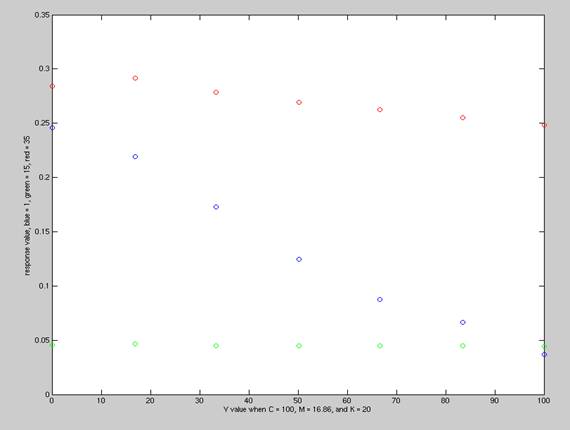
For example, let's fix the C,M and K values to some values and let's vary the Y values and plot the three reflectances for those different Y values from our database.

Here is what we obtain:

We can repeat this experiment several times fixing different values to gain the idea that we have a strong correlation between the reflectances and the CMYK values and that relationship seems to be linear.

In fact, after several model fitting experiments, the conclusion is that a log-linear model provide the best results. That is to say that for a given wavelength, we try to estimate the log value of the reflectance as a linear function of the C, M, Y, and K values.

Let's consider a typical example. We consider a specific wavelength (e.g. 560 nm) and we want to learn a log-linear model given the CMYK values. For this simulation purpose, we used the R programming language that provides the idea statistical toolbox.

Here is a summary of training a log-linear model on the provided data.

Call:

lm(formula = log(ref) ~ c + m + y + k)

Residuals:

Min 1Q Median 3Q Max

-2.58477 -0.09752 0.03014 0.13710 0.78169

Coefficients:

Estimate Std. Error t value Pr(>|t|)

Intercept -0.2882194 0.0201173 -14.33 <2e-16 ***

c -0.0041139 0.0002018 -20.39 <2e-16 ***

m -0.0100856 0.0002018 -49.99 <2e-16 ***

y -0.0175252 0.0002008 -87.28 <2e-16 ***

k -0.0206068 0.0002621 -78.61 <2e-16 ***

---

Signif. codes: 0 '***' 0.001 '**' 0.01 '*' 0.05 '.' 0.1 ' ' 1

Residual standard error: 0.251 on 1312 degrees of freedom

Multiple R-squared: 0.9562, Adjusted R-squared: 0.956

F-statistic: 4115 on 4 and 1312 DF, p-value: < 2.2e-16

What we can see from this summary of the model is that the R-squared error is very close to 1, the F-statistics very high and the p-value extremely small, proving that such a model fits very well our original database.

What we can also see is that the four values C,M,Y and K are important for our model ( all four are represented by ***, which means they are essential features of the model), which seems perfectly intuitive.

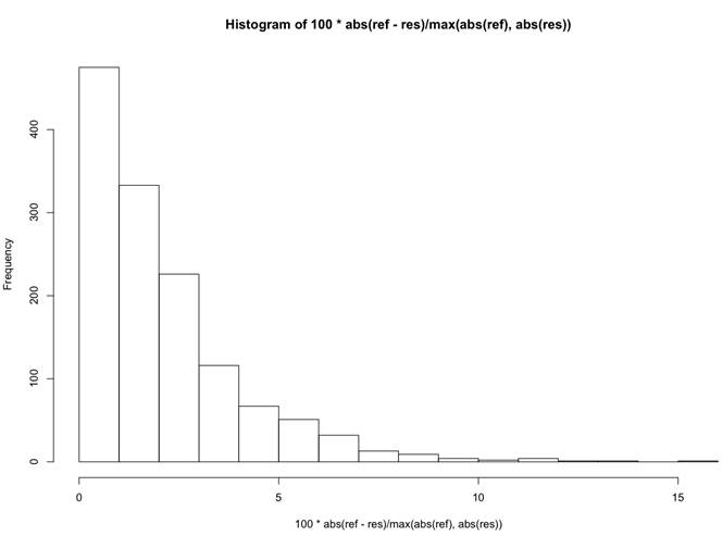
To see what it gives in term of error, let's have a look at the percentage of error for the CMYK values from the database with our model. Here is an histogram of the relative error:

What it shows is that for approximately 500 values (on 1338), the model gives an approximation of the reflectance that is within 1% of error from the exact value for a particular wavelength, which seems to be a good fit.

In we want to develop a real-time application, it might then be faster to use this kind of model, for which we only need 5 parameters per wavelength , so 5*35 parameters in total, which is much smaller than the original 1338 values needed for the locally linear model.

Scene model:

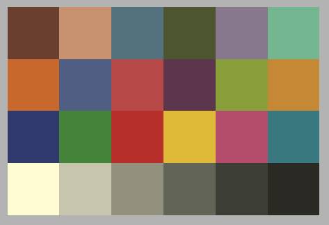
We can now take this map of reflectance and read it in ISET as we would read a Macbeth chart. We add a light. Now, from the reflectance, the light and the distance of the image, we can compute an ISET scene.

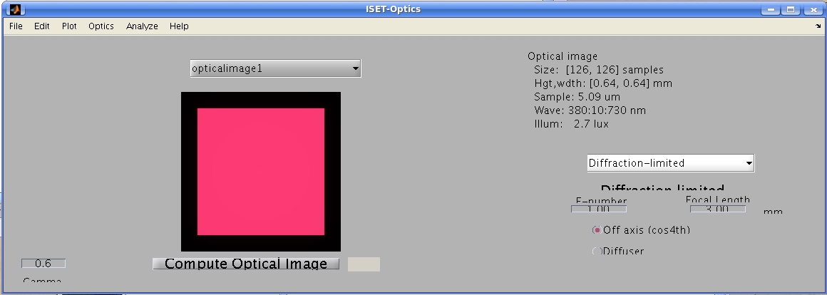
Optical image for a uniform patch:

Sensor model:

Now that we have determined the characteristics from experiment, we can fit them into ISET to simulate the sensor. We created quantum efficiency matrix based on the lab experiment and configurated the sensor model to fit with the measurements (PRNU, DSNU, dark current...)

This entire simulation process now provides a framework for simulation purposes. Let's take an example of an original image that we would like to print and measure visual information from it using our sensor and optics model.

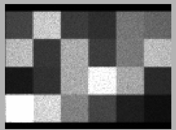
With our sensor and optics model, it is now easy to simulate the output for this given image :

What is interesting to see from a global perspective is that not all colors are discriminable. If you look at the patch on coordinates (2,2) and (3,2) or (1,5) and (2,5), the colors from the original Macbeth chart are perfectly discriminable. But, using this monochrome sensor makes them undiscriminable from the sensor images.

The goal then is to be able to provide some test results on which type of colors we are able to discriminate and also which type of spatial details we are able to capture with our entire system.