Call the output of the sensor when the black image is
applied, image A, and call the other one image B.
Test results
Mean of image A
is 0.0063 and the mean of image B is 0.0117. The standard deviation of image A
is
0.0029 and of
image B 0.0429.
Let’s look at
the mean values of the middle columns of image A formed by the sensor:
|
0.0067
|
0.0063
|
0.0068
|
0.0063
|
0.0067
|
0.0065
|
0.0062
|
0.0068
|
0.0066
|
And of image B:
|
0.0068
|
0.0069
|
0.008
|
0.077
|
0.4625
|
0.1615
|
0.0094
|
0.0063
|
0.0067
|
You can see that more
than 1 column averages are affected by a vertical line of 1 pixel
width. The difference of the highest
deviation mean (0.4625)
from the image
mean is around
10 standard deviations. Except these 2 central
columns, all other column means are within 1 standard deviation from the mean.

Test
conclusion
A white line at
a black background at this resolution (100x100) can be distinguished.
Test 3: Same as test 2 but image size is now increased to
200x200
Resizing the image has the following effect.
We are assuming that the image created in the computer takes the whole scene
width. Hence by increasing the image resolution, more information has to be fitted in
the same scene
width. This means
that it is
harder for the
sensor to discriminate spatial
differences of the same size as for an image of less resolution because
a line of one pixel width will spatially
take less distance in the paper.
Test results
The mean of the first
image is 0.0063 and the standard deviation is 0.0030 which are unchanged
from the lower resolution image.
The mean of the second image is 0.0081 and its standard deviation is
0.0160. Compared to the lower resolution
equivalent image, both the mean and the standard deviation have decreased,
which was expected since now the line
covers less pixels in the image.
Here are the
means of the middle columns of the first image formed in the sensor:
|
0.0064
|
0.0064
|
0.0064
|
0.0066
|
0.0066
|
0.0067
|
0.0069
|
0.0064
|
0.0065
|
Here are the
means of the middle columns of the second image formed in the sensor:
|
0.0069
|
0.0072
|
0.0066
|
0.0067
|
0.1743
|
0.0684
|
0.0072
|
0.0068
|
0.0067
|
The first thing you
can notice is that the maximum value here is 0.1743 (as opposed to 0.4625 in
the lower resolution image). The important thing to note here is that the deviation
of the maximum value from the mean value is still 10 standard deviations. In
addition, the large deviations from the mean no longer spread in a number of
columns but concentrate essentially to only one 1 sensor pixel width. All values
except the central column mean are within 1 standard deviation from the image
mean.
Test
Conclusion
The line can still be distinguished, but now the
width of the line it takes on the sensor image is much less. This indicates
that further increase of the image size, will make it harder and harder to
distinguish variations of one pixel width.
Test 4:
Decreasing the integration time
Test conditions
Integration time = 48/2770
Image size = 100
x 100
An image with black background and a white line is tested.
The integration time is halved.
Test results
Image mean is
0.0058 and the standard deviation is 0.0209. Here are the middle column means:
|
0.0038
|
0.0033
|
0.0043
|
0.0248
|
0.2261
|
0.0795
|
0.0043
|
0.0038
|
0.0037
|
0.0036
|
The white line here spans a 3 pixels width, and it
is again 10 standard deviations away from the mean.
Test conclusions
With integration time
48/2770 the line is still distinguishable.
Test 4:
Further Decreasing the integration time
Test
conditions
Integration time
= 12/2770
Image size = 100
x 100
An image with
black background and a white line is tested. The integration time is further
reduced.
Test results
Image mean is
0.0023 and the standard deviation is 0.0057. Both are reduced, compared to the
values obtained with a larger integration time.
These are the
means of the columns in the middle:
|
0.0013
|
0.0017
|
0.002
|
0.0096
|
0.0584
|
0.0207
|
0.0021
|
0.0016
|
0.0017
|
0.0014
|
The white line,
affects a width of 3 pixels. All values except the 3 central values are within
1 standard deviation from the mean.
Test
conclusions
With integration
time 12/2770 the line is still distinguishable.
Overall
Conclusion on above tests
Maximum and zero
intensity (e.g. black and white) images can be distinguished with a very high
spatial detail. For example, a white object which covers 1/200th of
the total area can be easily distinguished from the black background. In
addition, reducing the integration time to a small number, does not affect the
ability to distinguish black and white images. Hence, when the contrast is
large, we can be confident enough that we can infer very high spatial detail.
Parameter calculation for the real
case scenario
We currently know that the paper width
(which is the object width) is approximately 21.5 cm. This means that given
that the image width in the sensor is 128 pixels, the required resolution is

Hence the required magnification is

This defines the required image distance:

And hence the required focal length is:

Spatial testing
continues
Up to now, the tests have been run on the
system with default parameters. To add another level of realism to our tests,
it would be beneficial to actually consider the scene and optics properties in
more detail and recalculate the parameters in order to match our settings.
Calculating the field of view
Until now, we were forcing the scene
field of view to equal the sensor’s field of view. This ensures that the entire
scene width is seen by the sensor. This also means that given that the focal
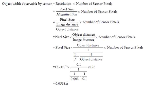
length was set to 0.003m and an object distance 0.1m the object width
observable by the sensor was

Which is verified by using the
command sceneGet(scene,'width').
Since we were forcing the field of view
of the scene to equal to this value, this means that by using the focal length
calculated in Camera Calculation we can set up our system to represent the
actual setting i.e. using f = 7.68×10⁴ m we are actually
able to match the actual scene width with the sensor width.
The
field of view
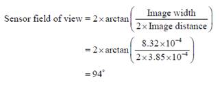
of the sensor
is calculated as
follows. Given the focal length f
=
7.68×10⁴ m and the
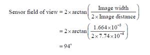
object distance is 0.1m then the image distance is 7.74×10⁴.
The image width is

And hence the field of view is

Which agrees with sensorGet(sensor,'fov').
Now let’s check that this field of view matches the field of view we
want to have for the scene. Given an object distance of 0.1m and given that the
object width is 21.5 cm (width of a page) then the scene field of view is

Wonderful! Both the sensor and the scene parameters have been
calculated so that they match the real setting. By changing the focal length of
the optics and forcing the FOV of the scene to match the FOV of the sensor, we
ensure that whole object width is observable by the sensor.
Testing without noise
It was suggested by experimental results, that the noise parameters
we are using in our script are probably set to too high values. So until we get
further results, it was suggested to turn off the noise parameters and test our
sensor simulator in a scheme that really describes “the best you can hope for”.
Tests
We would like to repeat some of the tests that have already been
done, in order to check the influence of changing the focal length to the value
that represents the real scenario. In addition the tests would now be carried
in absence of noise.
Relationship between image pixel
and sensor pixel
Let’s say we create an image on our computer of size x rows and y
columns. We are assuming that this image will take the whole scene width, i.e.
in this case 21.5 cm. For example, if the image has 100 columns, this means
that each pixel will take up 0.215 cm of space. We know from earlier
calculations that the resolution by which we are capturing the spatial
information is 1.67x10^-3 and hence we can calculate how many image pixels
correspond to sensor pixels by

I.e. we would expect that 1 image pixel will affect approximately 2 pixels.
In presence of noise or illumination effects the number sensor pixels changes.
Test 1: Comparing two black
images in the absence of noise
Test conditions
Integration time = 96/2770
Image size = 10 x 100
Both images are black
Test results
Output images of sensor have both mean 0.0036. Standard deviation of
both the images is 0.0098
Test conclusion
In the absence of noise, image
statistics are the same.
Test 2: Adding a vertical white
line to the black image
In important test is to be able to discriminate spatial differences.
We can add a vertical line in the middle of the image and see if we can
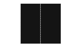
distinguish the line by using the image statistics. The image looks like this:

Test conditions
Integration time = 96/2770
Image size = 10 x 100
Black image with white vertical line
added in the middle.
Test results
The mean of the image is now 0.0050 (higher than before as
expected). The standard deviation is 0.0304 which is also higher than before.
The interesting sensor response lies in the middle (61-69) of the image. The
column averages are as follows:
|
0.0057
|
0.0061
|
0.0392
|
0.0853
|
0.0802
|
0.0063
|
0.0057
|
0.0058
|
0.0057
|
If we set to 0 all values that are within one standard deviation,
then the response is the following:
|
0.0000
|
0.0000
|
0.0392
|
0.0853
|
0.0802
|
0.0000
|
0.0000
|
0.0000
|
0.0000
|
This means that the white line has significantly affected the values
of 3 consecutive pixels. This is a bit higher than the expected number of influenced
pixels (which was 2).
Test conclusion
We can easily discriminate white lines of width 1 pixel from black
backgrounds when the width of the image is 100.
Test 3: Same as test 2 but image
size is now increased to 10x200
Note that now we are expecting the
vertical line to be affecting just one pixel.
Test results
The image mean is now 0.0022 and the
standard deviation is 0.0162. The middle column averages are now:
|
0.0029
|
0.0029
|
0.0029
|
0.0404
|
0.0172
|
0.0029
|
0.0029
|
0.0029
|
0.0029
|
And setting to 0 all values that are
within one standard deviation, then the response of the sensor is the
following:
|
0.0000
|
0.0000
|
0.0000
|
0.0404
|
0.0000
|
0.0000
|
0.0000
|
0.0000
|
0.0000
|
The white line is now affecting just
one pixel as expected.
Test Conclusion
Even at a higher image resolution, we can
still discriminate a white line from a black background.
Test 4: Same as test 3 but image
size is now increased to 10x400
Note that now we are expecting the
vertical line to be affecting around 0.3 pixels
Test results
The image mean is now 0.00086 and the
standard deviation is 0.0051. The middle column averages are now:
|
0.0014
|
0.0014
|
0.0014
|
0.0016
|
0.0022
|
0.0014
|
0.0014
|
0.0014
|
0.0013
|
And setting to 0 all values that are
within one standard deviation, then the response of the sensor is the
following:
|
0.00
|
0.00
|
0.00
|
0.00
|
0.00
|
0.00
|
0.00
|
0.00
|
0.00
|
The effect of the line has
disappeared!
Test Conclusion
At this resolution, we cannot distinguish
the vertical line. The vertical line occupies now just 1/400 of the total
width.
Further conclusion
The maximum image resolution at which we
can distinguish a single line was found to be at around 225.
Test 5: Discriminate two white
vertical lines Test conditions
Integration time = 96/2770 Image size =
10 x 100
One black image containing two white vertical lines. Each white line
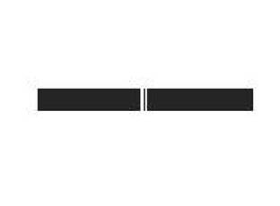
is one pixel wide and they are one pixel apart. The image looks like this:

Test results
The image mean is 0.0062 and the standard
deviation is 0.0405. The sensor response in the middle of the image is now:
|
0.0064
|
0.0810
|
0.0851
|
0.0288
|
0.0844
|
0.0836
|
0.0066
|
0.0057
|
0.005
|
And setting to 0 all values that are
within one standard deviation, then the response of the sensor is the
following:
|
0.0000
|
0.0810
|
0.0851
|
0.0000
|
0.0844
|
0.0836
|
0.0000
|
0.0000
|
0.0000
|
Each white line is affecting 2
pixels and they are spaced one pixel apart.
Test conclusion
The two lines can be distinguished
at this image resolution.
Test 6: Same as test 5 but now
the image size is set to 10x200
Test results
The image mean is 0.0024 and the standard
deviation is 0.0213. The sensor response in the middle of the image is now:
|
0.0029
|
0.0029
|
0.0030
|
0.0039
|
0.0431
|
0.0438
|
0.0036
|
0.0030
|
0.0029
|
And setting to 0 all values that are
within one standard deviation, then the response of the sensor is the
following:
|
0.0000
|
0.0000
|
0.0000
|
0.0000
|
0.0431
|
0.0438
|
0.0000
|
0.0000
|
0.0000
|
Test conclusion
The one pixel separation has now
disappeared. The two lines now appear as one thicker line. Hence it is
impossible to distinguish two lines spaced one pixel apart at this image
resolution.
Changing the sensor resolution
Up to this point the tests have been performed by representing the
object width (21.5cm) with 128 pixels. An important test would be how well we
can do with less available pixels. The current resolution is hence:

What if we had half the pixels available? Then the resolution would be

And hence the magnification is

And the image distance is:

And let’s check that the sensor
field of view is also fine:
The image width is

And hence
the sensor field of view is

So everything is compatible again!!
For each of
the following tests, the focal length is calculated accordingly.
Test 7: Adding a vertical white
line to the black image, sensor image width 64 pixels
Test conditions
Integration time = 96/2770
Image size = 10 x 100
Black image with white vertical line
added in the middle.
Sensor pixel positions available in
width = 64
Test results
The mean of the image is now 0.0026. The standard deviation is
0.0218. The interesting sensor response lies in the middle (28-36) of the
image. The column averages are as follows:
|
0.0028
|
0.0028
|
0.0028
|
0.0029
|
0.0403
|
0.0172
|
0.0029
|
0.0028
|
0.0028
|
If we set to 0 all values that are within one standard deviation,
then the response is the following:
|
0.0000
|
0.0000
|
0.0000
|
0.0000
|
0.0403
|
0.0000
|
0.0000
|
0.0000
|
0.0000
|
This means that the white line has significantly affected the values
of 1 pixel. The expected number of sensor pixels affected was 0.64 pixels.
Test conclusion
We can discriminate white lines of width 1 pixel from black
backgrounds when the width of the image is 100 and the sensor width is 64
pixels.
Test 8: Adding a vertical white
line to the black image, sensor image width 32 pixels
Test conditions
Integration time = 96/2770
Image size = 10 x 100
Black image with white vertical line
added in the middle.
Sensor pixel positions available in
width =32
Test results
The mean of the image is now 0.00089. The standard deviation is
0.0054. The interesting sensor response lies in the middle (12-20) of the
image. The column averages are as follows:
|
0.0011
|
0.0012
|
0.0013
|
0.0014
|
0.0016
|
0.0022
|
0.0014
|
0.0013
|
0.0013
|
If we set to 0 all values that are within one standard deviation,
then the response is the following:
|
0.0000
|
0.0000
|
0.0000
|
0.0000
|
0.0000
|
0.0000
|
0.0000
|
0.0000
|
0.0000
|
This means that the white line has not affected any pixels. The
relationship of sensor pixel to image pixel here is

So the result makes sense.
Test conclusion
We are not able to discriminate white lines of width one pixel given
32 sensor pixels and an image of width 100 pixels.
Test 9: Same as test 8 but now
the sensor pixels are increased to 512
Test conditions
Integration time = 96/2770
Image size = 10 x 100
Black image with white vertical line
added in the middle.
Sensor pixel positions available in
width = 512

Test results
The mean of the image is now 0.0273. The standard deviation is
0.0569. The interesting sensor response lies in the middle (252-260) of the
image. The column averages are as follows:
|
0.3340
|
0.3384
|
0.3411
|
0.3397
|
0.3360
|
0.3294
|
0.2674
|
0.0810
|
0.0231
|
If we set to 0 all values that are within one standard deviation,
then the response is the following:
|
0.3340
|
0.3384
|
0.3411
|
0.3397
|
0.3360
|
0.3294
|
0.2674
|
0.0000
|
0.0000
|
This means
that the white line has significantly affected the values of more than 7 pixels
(it’s actually 9). The expected number of sensor pixels affected was 5.12
pixels. It would be also nice to see how many pixels are more than five
standard deviations from the mean:
|
0
|
0.325293
|
0.33405
|
0.338404
|
0.341083
|
0.339664
|
0.335994
|
0.32942
|
0
|
The non-zero terms have decreased to
7.
Test conclusion
We can discriminate white lines of width 1 pixel from black
backgrounds when the width of the image is 100 and the sensor width is 512
pixels.
Test 10: Same as test 9 but now
the sensor pixels are increased to1024
Test conditions
Integration time = 96/2770
Image size = 10 x 100
Black image with white vertical line
added in the middle.
Sensor pixel positions available in
width = 1024

Test results
The mean of the image is now 0.0487. The standard deviation is
0.0694. After setting to zero all values that were within 1 standard deviation,
20 pixels remained non-zero (the central ones)
Test conclusion
We can discriminate white lines of width 1 pixel from black
backgrounds when the width of the image is 100 and the sensor width is 1024
pixels
![]()
![]()
![]()
![]()
![]()

